Personal web pages of

Tim Stinchcombe

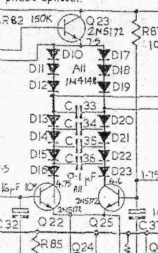
Diode Ladder Filters

[Update 02 Aug 2010: Since I receive quite a lot of hits from various forum discussions about the relative merits of Roland filters, and their different topologies, I thought I would include a link to Florian Anwander's useful summary page of Roland filters, just for reference—there is much interesting and useful information there!]

[Update 14 Dec 2009: I have generated a new page containing some extra data relating to the big transfer function below.]

[Update 19 Jul 2009: Here is the transfer function I finally ended up with—it turned out to have 10 poles and six zeroes: \begin{multline*} H(s)=\dfrac{1.06s^3(s+109.9)(s+34.0)(s+7.41)}{\left(\dfrac{s^4}{\omega_c^4}+2^{\frac{11}{4}}\dfrac{s^3}{\omega_c^3}+10\sqrt{2}\dfrac{s^2}{\omega_c^2}+2^{\frac{13}{4}}\dfrac{s}{\omega_c}+1\right)(s+97.5)(s+38.5)(s+4.45)}\cdots\\ \cdots\frac{\phantom{1}}{\rule[-2mm]{0mm}{8mm}\times(s+578.1)(s+20.0)(s+7.41)+18.7ks^4(s+46.5)(s+4.40)} \end{multline*} Note that it is highly non-normalized; \(\omega_c\) is as for \(H_{tb}\) below, and \(k\) is the resonance (and please excuse the clumsy 'line wrap'—I don't think LaTeX has a standard way to do that...). I must stress that this is all based on SPICE simulation, so take it for what its worth: I was hoping to check its veracity against some real hardware, an Analogue Solutions TBX-303, a TB-303 clone, but I had some niggly little problems doing so, and thus I temporarily shelved working on this some time ago (the problems have been overcome now though).]

[Update 19 Feb 2009: I am continuing to look at the TB-303 filter in greater detail, concentrating on the high-pass effects that all the coupling caps around the feedback loop introduce. It is clear that not accounting for them, as this and the filter pole animations page currently do, is to miss out on some very significant affects, as they turn the transfer function into a nine-pole monstrosity, with five new zeroes to match. The five new poles are all clustered at a low frequency, around 10Hz or so, and as such do not materially affect the conclusions drawn on the main low-pass effects presented in these pages (though they do make the main resonant peak frequency-dependent). However, as most are inside the feedback loop, they create another resonant peak at this frequency, and I feel the effects of this must reach into the audible range, so to neglect them (in any digital implementation, say) is likely to miss out on some of the character of the filter. Hopefully in a few weeks I will be able to make available a small summary of what I've learned so far, with a more comprehensive treatment to follow later!]

[Update 26 Oct 2008: I have now updated my Moog ladder paper, and it does now include the derivation of the transfer functions of (some of) the diode ladder filter variants.]

The success of the Moog transistor ladder filter quickly gave rise to a number of 'look-alikes', which employed diodes in the ladder in order to circumvent the Moog patent. Two of the better-known examples are the Roland TB-303 filter:

and the EMS filter, as used in the VCS3 (and probably other models)—this is the 4-pole '18dB' one; later filters had 5 poles, and were labelled '24dB':

Notice that there are small differences between the two: the EMS filter has a chain of three diodes at the top of each arm of the ladder, and all capacitor values are equal; in the TB-303 the lowest capacitor is half the value of the other three, and at the top of the ladder is a single pair of transistors, biased at a common point, which effectively act like a single diode in each arm of the ladder.

Aside from these differences, superficially they both look similar to the transistor ladder filter structure, but the move from transistors to diodes has implications in the way the circuit operates, and in one sense this leads to the loss of a certain amount of 'elegance' too: the resistor chain used to bias the transistors in the Moog ladder means that the voltages at each filter section are separated, which effectively means that the sections are buffered from each other; this 'isolation' is simply not present in the diode ladder, giving it a quite different transfer function (it is much harder to derive), and which in turn means the pole placement and their subsequent movement with increasing resonance is also quite different from the transistor version.

Deriving the transfer function requires a good deal of tedious algebraic manipulation, and is incredibly error-prone. I also increased the number of terms that needed tracking through all the manipulation by introducing quantities which helped keep it more general. With: \(C_1\) the value of the lowest capacitor in the ladder; \(C\) the other three capacitors; \(d\) the number of diodes in the chain at the top of each arm; \(a\) substituted as

for convenience, where \(V_T\) is the usual thermal voltage and \(I_f\) the current drawn out the bottom of the ladder (which defines the cut-off frequency), it is possible to arrive at the following general expression for the transfer function \(H(s)\) (which I've inverted to rid the nasty long fraction):

(Note that this is just for the ladder 'core' itself—no feedback or resonance is involved here.) If we take the simplest case (not shown here) of one diode at the top, and all capacitors equal, i.e. \(d = 1\) and \(C_1 = C\), this will give

Equating the coefficient on the highest order term in the denominator as

so that we get

then the expression becomes

and which when normalized finally becomes

Some plots of the poles of this function are to be found on the filter pole animations page. It has been derived elsewhere (diligent searching of the web and the Synth DIY archives will probably uncover it), and it is the one most normally given as the 'transfer function of a diode ladder filter'—however it is not the full story.

and this time put

so that

and then normalize and evaluate the constants to finally get

The denominator of this isn't a million miles away from that of \(H_1\) above, but note that all the poles have moved, but some by only a small amount:

\(H_1\) poles: (-3.53,0), (-2.35,0), (-1.00,0), (-0.12,0)

\(H_{tb}\) poles: (-3.24,0), (-2.33,0), (-1.04,0), (-0.13,0)

Intuitively, halving the bottom capacitor should increase the cut-off frequency, as the smaller cap value has a greater impedance, and so more of the signal (at a fixed frequency) should make it up the ladder, rather than being shorted through the cap. This is borne out by the analysis: eliminate \(aC\) between the two \(\omega_c\) expressions, and it can be seen that that for \(H_{tb}\) is \(2^{0.25} = 1.189\) times that for \(H_1\). To further convince myself of the efficacy of my analysis, I did the following: I entered the core part of the TB-303 filter into SIMetrix, only I set all four capacitors to the same value, 33nF, and ran an AC analysis at one particular cut-off frequency; exported the plot data to Excel, and multiplied the frequency component by 1.189; re-imported the data into SIMetrix, and added the curve to the plot; halved the bottom capacitor, setting it to 16.5nF, and ran another analysis. The following plot shows the result: the trace predicted by the analysis 'correction', and the second simulation run are nearly identical:

Zooming in on part of the plot shows that indeed there really are three traces in there:

Plotting both the normalized responses of \(|H_1(\omega j)|\) and \(|H_{tb}(\omega j)|\) (via Mathematica) shows just how close they are—the red trace is \(H_1\), with the equal capacitors, the blue is \(H_{tb}\), with the bottom cap halved, as the TB-303:

Zooming in a little again shows just how little there is to choose between the two:

My point in all this? My suspicions are that halving the lowest capacitor is not based on any aural consideration of how the filter sounds. One often sees comments to the effect that 'halving the lowest capacitor moves that section's pole up an octave'. Well yes and no: 'yes', because as mentioned above, the overall frequency response will shift upwards; 'no' in that there is no simple relationship between each filter section and the poles. This is because there is no buffering between each section, and so it is not possible to consider them in isolation. This is also borne out by the comparison of pole values above: after re-normalization, any such 'doubled' pole would appear as \(\times 1.682\; (=2^{0.75})\), and the other three as \(\times 0.841\; (=2^{-0.25})\) their old values, and there is clearly no such relationship seen between the poles above. Certainly, if you were to arrange a filter with capacitors that could be switched between half and full value, then you probably would feel that it sounded different at the different switch positions, but from this analysis, changing the bottom cap is closely equivalent to shifting the whole response of the filter up or down in frequency, merely doing the same as if you had adjusted the offset pot which sets the relative position of the cut-off frequency (assuming such a pot exists, which is very likely). If you took two otherwise identical filters, but one with the bottom cap halved, the other not, and calibrated them both to have the same cut-off at the same CV in, then I suspect you would have to work pretty hard to tell which is which from the sound of the filters alone.

I think the reason for halving the capacitor is more likely to be some sort of stability consideration: whilst running SPICE simulations in SIMetrix in preparation for this page, I noticed that at high frequencies (low MHz and above), something horrid was happening, which is odd since they were mostly AC analyses, and in my experience it is a lot harder to upset a SPICE AC analysis when compared to, say, a transient analysis. However I have not been able to spend much time on what the cause of the apparent instability in the simulation is, so I really do not know. 14.12.09: I'm reasonably certain that what I was seeing was numerical instability in the simulation: in order to ignore the unwanted effects of coupling capacitors one often makes them ludicrously large—terafarads for example—but then this can cause numeric problems, due to trying to cope with both stupidly large and normal, picofarad-sized values.

The later '24dB' EMS filter: this seems like good a point to mention this filter. (My analysis here is based on the Analogue Solutions RS500e 'authorized copy' of this filter—I have not seen any actual EMS schematics of this variant, but the 18dB variant does match the VCS3 schematics I have seen very closely, so I have no reason to believe that the 24dB version deviates in any significant way from the EMS original.) The '24dB' variant is actually a 5-pole filter, so nominally 30dB/octave attenuation in the stopband: however this is achieved by stringing a 100Ω resistor in series with a 100nF capacitor between the cathodes of the bottom pair of diodes in the ladder (D16 and D23 in the image above). The extra capacitor gives the fifth pole, but the effect of the resistor is to introduce a zero into the numerator of the transfer function, at approximately 16kHz. Thus the 30dB attenuation gets turned back up to 24dB before it really gets going—this is all happening above the useful audio range, so I again feel this must be for some sort of stability reason, and nothing to do with any kind of aural consideration of how the filter sounds (and again, I have not had the time to investigate this premise any further).

Returning now to the transfer function of the (early) EMS filter, put \(d = 3\) and \(C_1 = C\) in the general form, reflecting the equal value capacitors and the three diodes at the top:

and this time we put

so that

and again normalize and evaluate the constants to get

The effect of \(d = 3\), i.e. the three diodes in the chain at the top of the ladder, is most apparent by the increased gain, the '3' in the numerator, and the coefficients are now markedly different from before. If we ignore the extra gain, plots of \(H_1\) (red), and \(H_{ems}\) (blue) do now show some difference:

[I nearly entitled this section 'debate', but that is not really a good word to use here—there simply is no debate: these filters are 4^th-order, 4-pole, 24dB/octave attenuation low-pass filters, plain and simple.]

Start reading about the Roland TB-303 and it will not be long before you come across mention of its '18dB 3-pole lowpass filter'—apparently even Roland themselves described the filter as having these properties. A similar story could also be told of the early EMS filter. One can only guess at the motives of both Roland and EMS for doing so: high on the list would be that this reasonably well describes the behaviour of the filter, in that the transition from the passband to stopband starts earlier, and lasts longer than, the (then) more-usual 4-pole filter (such as the Moog transistor ladder), so that the 'corner' in the frequency response is altogether a less pronounced affair (comparison plots and animations); another reason might be to try and highlight the fact that these filters are different from the competition's filters, and hence by implication, better in some way; less likely is the idea that they would want the filters to be seen as different from the Moog ladder from the patent-infringement point of view (one would expect patent lawyers to be better informed than to be taken in by this). But whatever the reasons, these filters simply are not 18dB 3-pole filters: by all means they could be described as behaving more like 18dB/octave, rather than 24dB/octave, in the main region in which they are used (this could be said of many other filters though, yet isn't), but they simply cannot escape the fact that they are 4^th-order, 4-pole, 24dB/octave filters, and calling them anything else is at best misleading, and at worse, just plain incorrect. If you owned a Porsche 911, but only drove it at 40mph to pick up the shopping on a Saturday afternoon, and somebody asked you what it is, you wouldn't say "it is a Saturday run-around", you'd probably say something like "it is a 150mph+ high-performance sports car", or maybe even "it is a 150mph+ high-performance sports car, but generally I only use it as a Saturday run-around"—just because you don't use it for what it was normally intended doesn't stop it being what it is.

Impact of the fourth pole. There was a little dialogue over at reddit.com as to whether the impact of the largest pole is mostly above the frequency where the response drops below the 'noise floor' of the filter, and hence possibly why this pole could be 'discarded', with the filter being regarded as '18 dB'. It is a relatively simple matter to plot the frequency response of just the three lower poles, and to compare this against the 4-pole version: in the following plot the blue curve is of the function \(H_{tb}\) given above (i.e. with all poles present), and the red trace is that formed when the largest pole, (-3.24,0), is omitted (and having been re-normalized)—it is quite apparent that due to the closeness of the fourth pole to all the others, it is making a significant contribution to the overall shape of the response, at frequencies well inside the region of interest, and so it shouldn't be ignored:

So how many ways can we tell that these filters are 24dB/octave?:

1. Count the sections:

So 4 sections, 6dB/octave each gives 4 x 6 = 24dB/octave.

2. Do some SPICE simulations: from a simplified circuit of the core of the TB-303 filter (schematic here for the more curious), here is a (rather busy) plot from SIMetrix of the output from each stage as we go up the ladder:

The vertical mauve lines are at approximately 61kHz and 122kHz, i.e. an octave apart (arbitrarily chosen so that the horizontal lines didn't clash with any grid lines). The following table gives the values of the y-intercepts of each curve where they cut the mauve lines, and hence the resulting gradients:

3. Do some analysis: work out the transfer function, and find the highest order of \(s\) in the denominator. For example:

We observe that it is 4, so fourth-order. If we want to know how much the signal is attenuated an octave above some frequency \(\omega_1\), say, we need to calculate:

For \(\omega_1\) well into the stopband, it can be shown that it is this highest order term in the denominator that dominates, hence we can approximate as

which simply evaluates as

Yet again, we see we get 24dB/octave.

4. Plot the transfer function: take the transfer function from the step above, and plot the amplitude function \(|H_{tb}(\omega j)|\):

The horizontal red lines intersect the curve at -94.4 and -118.3, giving the gradient, yet again, as -118.3-(-94.4) = -23.9dB/octave.

Yep, they look like 24dB/octave, 4-pole filters to me. QED.

Sines of Reality

In volume 4, issue 18, of The Institution of Engineering and Technology's Engineering & Technology magazine, I made a small contribution to an article that reports on attempts to emulate analogue hardware digitally, the TB-303 getting a particular mention: Sines of Reality, Vol 4, Issue 18, 24 Oct-6 Nov 2009, pp32-35.

[Page last updated: 17 Dec 2022]